
by Brendan O’Flaherty, CEO, cPacket Networks
The 100Gbps Ethernet transport network is here, and the use cases for transport at 100Gbps are multiplying. The previous leap in network bandwidths was from 10Gbps to 40Gbps, and 40Gbps networks are prevalent today. However, while 40Gbps networks are meeting bandwidth and performance requirements in many enterprises, the “need for speed” to handle data growth in the enterprise simply cannot be tamed.
As companies continue to grow in scale, and as their data needs become more complex, 100Gbps (“100G”) offers the bandwidth and efficiency they desperately need. In addition, 100G better utilizes existing fiber installations and increases density, which significantly improves overall data center efficiency.
A pattern of growth in networks is emerging, and it seems to reflect the hypergrowth increases in data on corporate networks just over the last five years. In fact, the now-famous Gilder’s Law states that backbone bandwidth on a single cable is now a thousand times greater than the average monthly traffic exchanged across the entire global communications infrastructure five years ago.
A look at the numbers tells the story well. IDC says that 10G Ethernet switches are set to lose share, while 100G switches are set to double. Crehan Research (see Figure 1) says that 100G port shipments will pass 40G shipments in 2017, and will pass 10G shipments in 2021.

Figure 1: 100G Port Shipments Reaching Critical Mass, as 40G and 10G Shipments Decline
The increase in available link speeds and utilization creates new challenges for both the architectures upon which traditional network monitoring solutions are based and for the resolution required to view network behavior accurately. Let’s look at some numbers:
100G Capture to Disk
Traditional network monitoring architectures depend on the ability to bring network traffic to a NIC and write that data to disk for post-analysis. Let’s look at the volume of data involved at 100G:
By equation (3), at 100 Gbps on one link, in one direction, a one-terabyte disk will be filled in 80 seconds. Extending this calculation for one day, in order to store the amount of data generated on one 100 Gbps link in only one direction, 0.96 petabytes of storage is required:
 |
(4) |
Not only is this a lot of data (0.96 petabytes is about 1,000 terabytes, equivalent to 125 8TB desktop hard drives), but as of this writing (Aug 2017), a high-capacity network performance solution from a leading vendor can store approximately 300 terabytes, or only eight hours of network data from one highly utilized link.
100G in the Network – What is a Burst, and What is Its Impact?
A microburst can be defined as a period during which traffic is transmitted over the network at line rate (the maximum capacity of the link). Microbursts in the datacenter are quite common – often by design of the applications running in the network. Three common reasons are:
- Traffic from two (or more) sources to one destination. This scenario is sometimes considered uncommon due to the low utilization of the source traffic, although this impression is the result of lack of accuracy in measurements, as we’ll see when we look at the amount of data in a one-millisecond burst.
- Throughput maximizations. Many common operating system optimizations to reduce the overhead of disk operations or NIC offloading of interrupts will cause trains of packets to occur on the wire.
- YouTube/Netflix ON/OFF buffer loading. Common to these two applications but frequently used with other video streaming applications is buffer loading from 64KB to 2MB – once again, this ON/OFF transmission of traffic inherently gives rise to bursty behavior in the network.
The equations below translate 100 gigabits per second (1011 bits/second) into bytes per millisecond:
 |
(5)
|
 |
(6)
|
The amount of data in a one-millisecond spike of data is greater than the total amount of (shared) memory resources available in a standard switch. This means that a single one-millisecond spike can cause packet drops in the network. For protocols such as TCP, the data will be retransmitted; however, the exponential backoff mechanisms will result in degraded performance. For UDP packets, the lost packets will translate to choppy voice or video, or gaps in market data feeds for algorithm trading platforms. In both cases, since the packet drops cannot be predicted in advance because the spikes and bursts will go undetected without millisecond monitoring resolution, the result will be intermittent behavior that is difficult to troubleshoot.
Network Monitoring Architecture
Typical Monitoring Stack
The typical network monitoring stack is described in Figure 2. At the bottom is the infrastructure – the switches, routers and firewalls that make up the network. Next, in the blue layer are TAPs and SPAN ports – TAPs are widely deployed due to their low cost, and most infrastructure devices provide some number of SPAN ports. The traffic from these TAPs and SPANs is then taken to an aggregation device (or matrix switch or “packet broker”) – at this point, a high number of links, typically 96 10G, are taken to a small number of tool ports, usually four 10G ports (a standard high-performance configuration). At the top are the network tools – these tools take the network traffic fed to them from the aggregation layer and provide the graphs, analytics and drilldowns that form dashboards/visualization.

Figure 2: Typical Network Monitoring Stack
Scalability of Network Monitoring Stack
Let’s now evaluate how this typical monitoring stack scales in high-speed environments.
· Infrastructure: As evidenced by the transition to 100G, the infrastructure layer appears to be scaling well.
· TAP/SPAN: TAPs are readily available and match the speeds found in the infrastructure layer. SPANs can be oversubscribed or alter timing, leading to loss of visibility and inaccurate assumptions about production traffic behavior.
· Aggregation: The aggregation layer is where the scaling issues become problematic. As in the previous example, if 48 links are monitored by four 10G tool ports, the ratio of “traffic in” to monitoring capability is 96:4 (96 is the result of 48 links in two directions) or, reducing, an oversubscription ratio of 24:1. Packet drops due to oversubscription mean that network traffic is not reaching the tools – there are many links or large volumes of traffic that are not being monitored.
· Tools: The tools layer is dependent on data acquisition and data storage, which translates to the dual technical hurdles of capturing all the data at the NIC as well as writing this data to disk for analysis. Continuing the example, at 96x10G to 4x10G at 10G, the percentage of traffic measured (assuming fully utilized links) is 4x10G/96x10G, or 4.2%. As the network increases to 100G (but the performance of monitoring tools does not), the percentage of traffic monitored drops further to 4x10G/96x100G, or 0.42%.
It is difficult to provide actionable insights into network behavior when only 0.42% of network traffic is monitored, especially during levels of high activity or security attacks.
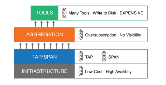
Figure 3: Scalability of Network Monitoring Stack
Current Challenges with Traditional Monitoring Environments
Monitoring Requirements in the Datacenter
Modern datacenter monitoring has a number of requirements if it is to be comprehensive:
- Monitoring Must Be Always-On. Always-on network performance monitoring means being able to see all of the traffic and being able to perform drill-downs to packets of interest on the network without the delay incurred in activating and connecting a network tool only after an issue has been reported (which leads to reactive customer support rather than the proactive awareness necessary to address issues before customers are affected). Always-on KPIs at high resolution provide a constant stream of information for efficient network operations.
- Monitoring Must Inspect All Packets. To be comprehensive, NPM must inspect every packet and every bit at all speeds—and without being affected by high traffic rates or minimum-sized packets. NPM solutions that drop packets (or only monitor 0.24% of the packets) as data rates increase do not provide the accuracy, by definition, to understand network behavior when accuracy is most needed – when the network is about to fail due to high load or a security attack.
- High Resolution is Critical. Resolution down to 1ms was not mandatory in the days when 10Gbps networks prevailed. But there’s no alternative today: 1ms resolution is required for detecting problems such as transients, bursts and spikes at 100Gbps.
- Convergence of Security and Performance Monitoring (NOC/SOC Integration). Security teams and network performance teams are often looking for the same data, with the goal of interpreting it based on their area of focus. Spikes and microbursts might represent a capacity issue for performance engineers but may be early signs of probing by an attacker to a security engineer. Growing response time may reflect server loads to a performance engineer or may indicate a reflection attack to the infosec team. Providing the tools to allow correlation of these events, given the same data, is essential to efficient security and performance engineering applications.
100G is just the latest leap in Ethernet-based transport in the enterprise. With 100G port shipments growing at the expense of 40G and 10G, the technology is on a trajectory to become the dominant data center speed by 2021. According to Light Reading, “We are seeing huge demand for 100G in the data center and elsewhere and expect the 100G optical module market to become very competitive through 2018, as the cost of modules is reduced and production volumes grow to meet the demand. The first solutions for 200G and 400G are already available. The industry is now working on cost-reduced 100G, higher-density 400G, and possible solutions for 800G and 1.6 Tbit/s.”


